Lesson 5 — Intermediate

Seaborn se Statistical Plots — Heatmap aur Regression

Matplotlib me sab manually set karna padta hai. Seaborn ek function me title, palette, grid aur statistics ke smart defaults de deta hai. Is lesson me do powerhouse plots banayenge — correlation heatmap aur regression scatter.

⏱ 25 min• Intermediate• Jupyter / Colab

Seaborn vs Matplotlib

WHAT

Seaborn = Matplotlib ka statistical wrapper. Default palettes, automatic legends, DataFrame column names se direct plotting (x="col") — 5 line me complete chart.

WHEN

EDA me: correlation dekhna, category distributions compare karna, relationship + uncertainty (CI) dikhana. Publication-grade stats plots quick banane ho.

WHERE

EDA reports, deck visuals, ML assumption checks (multicollinearity heatmap). Seaborn ka output Matplotlib axes hi hai — customisation sab possible rehti hai.

Theme setup

import seaborn as sns
import matplotlib.pyplot as plt

sns.set_theme(style="darkgrid", palette="viridis")

# Dark custom theme (jaise hum use karte hain)
BG = "#0d0d1c"
sns.set_theme(style="whitegrid", palette="deep")
plt.rcParams.update({
    "figure.facecolor": BG, "axes.facecolor": BG,
    "axes.edgecolor": "rgba(255,255,255,.2)",
    "axes.labelcolor": "#8a8aa3", "text.color": "white",
    "xtick.color": "#8a8aa3", "ytick.color": "#8a8aa3",
    "grid.color": "rgba(255,255,255,.08)",
    "font.family": "sans-serif"})

# Palette: 3 colours jo hamare brand se match karte hain
PALETTE = ["#f0a500", "#8b5cf6", "#2dd4bf"]
sns.set_palette(PALETTE)

Correlation heatmap

import pandas as pd
import numpy as np

np.random.seed(7)
data = pd.DataFrame({
    "ad_spend":   np.random.rand(300) * 50,
    "price":      500 + np.random.rand(300) * 300,
    "delivery_h": np.random.rand(300) * 10})
# relationships inject karte hain
data["sales"] = (data["ad_spend"] * 8 - data["price"] * 1.5
                 - data["delivery_h"] * 12 + np.random.randn(300) * 20 + 400)

corr = data.corr(numeric_only=True)

fig, ax = plt.subplots(figsize=(8, 6), facecolor=BG)
sns.heatmap(corr, annot=True, fmt=".2f", cmap="viridis",
            linewidths=1, linecolor=BG, ax=ax,
            annot_kws={"size": 11})
ax.set_title("Feature Correlation Matrix", color="white", fontsize=15)
plt.tight_layout(); plt.show()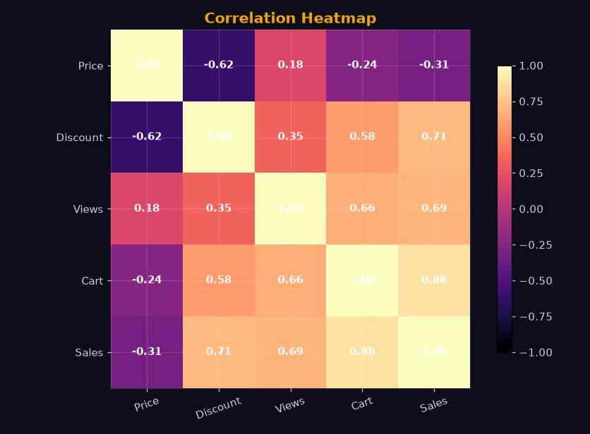

Scatter + regression line

fig, ax = plt.subplots(figsize=(9, 5), facecolor=BG)
sns.regplot(data=data, x="price", y="sales",
            scatter_kws={"alpha": 0.45, "color": "#2dd4bf", "s": 42},
            line_kws={"color": "#f0a500", "linewidth": 2.5},
            ax=ax)
ax.set_title("Price vs Sales (with 95% CI)", color="white", fontsize=15)
ax.set_xlabel("Price (₹)", color="#8a8aa3")
ax.set_ylabel("Sales", color="#8a8aa3")
plt.tight_layout(); plt.show()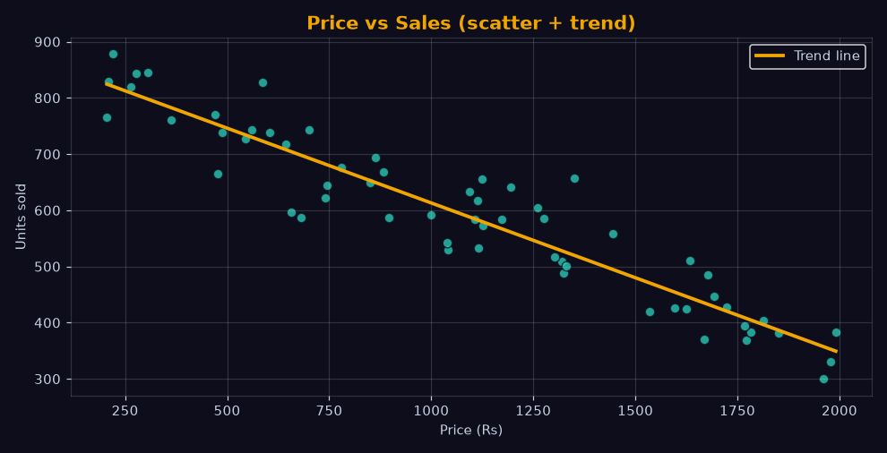

Price versus sales scatter plot with gold regression line and confidence band on dark background — Scatter plot — price vs sales + regression line (confidence band ke saath)

Plot selection — quick reference

corr mat → sns.heatmap(corr, annot=True)
do numeric ka relationship → sns.regplot (line + CI), sirf points → sns.scatterplot
category distribution → sns.boxplot / sns.violinplot
count per category → sns.countplot
pairwise relations → sns.pairplot(df) (EDA ka shortcut)
time trend multi-series → sns.lineplot(data=df, x="date", y="v", hue="city")

Reading a heatmap: Correlation +1 = saath saath badhta hai, -1 = ulta, 0 = koi relation nahi. Heatmap me |0.7|+ wale pairs dhundo — multicollinearity (do features ek hi baat keh rahe hain) wahi hoti hai jo model ko confuse karti hai.

Exercise

Question: Correlation matrix ko color blocks me dikhane wala seaborn plot? (7 letters)

Question: Scatter ke saath regression line khud draw karne wala seaborn function? (7 letters)

Common mistakes

annot ke bina heatmap: Values na ho to interviewer number padh nahi pata — EDA me annot=True default rakho.
Poor color choice: Rainbow/viridis heatmap achhi, red-green colorblind-hostile combos avoid karo.
Overplotting: 50k points ke scatter me alpha (transparency) do warna solid block ban jaata hai.
CI miss: regplot ka band 95% confidence hai — report me isi ko "statistical strength" kehte hain.

Interview question: "Correlation aur causation me farak?" — Correlation = dono saath chalte hain; Causation = ek doosre ko cause karta hai (randomization/experiment chahiye proof ke liye). Ice-cream aur drowning dono summer se correlate, ice-cream drowning nahi karti.

Lesson complete?

Lesson ho gaya? Ab next pe chalte hain — Sales EDA Project.